Skewness, Kurtosis and Normality Checks

Where this fits

Continues from The Normal Distribution. Real data is rarely perfectly normal. This note covers the two shape measures that quantify the departure from normal, skewness (asymmetry) and kurtosis (tail heaviness), and then the practical tools for checking whether data is normal, culminating in the QQ plot.

---

Skewness

Skewness measures the asymmetry of a distribution, i.e. how far it deviates from being symmetric (normal). High skewness means the data is not normally distributed.

• A skewed distribution has one tail longer than the other. Since a tail represents outliers, you always name the skew after the side the tail is on.

Type	Tail is longer on the	Order of measures
Positive (right) skew	right	mode < median < mean
Symmetric	both equal	mean = median = mode
Negative (left) skew	left	mean < median < mode

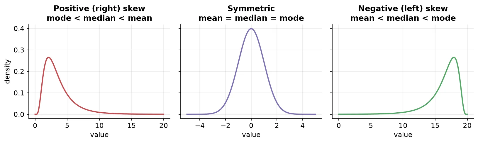
The mean gets pulled toward the tail (the outliers). The greater the skew, the greater the distance between the mean and the mode/median. With no skew they sit on top of each other.

Formula (statistical moments)

Statistics has a sequence of “moments”: the 1st moment is the mean, the 2nd is variance, the 3rd is skewness, and the 4th is kurtosis. Sample skewness:

$$\text{Skew} = \frac{n}{(n-1)(n-2)} \sum \left(\frac{x_i - \bar{x}}{s}\right)^3$$

You rarely compute this by hand; df.skew() in pandas or Excel’s SKEW does it. What matters is interpreting the number.

Interpreting the skew value

   highly     moderately   almost      moderately    highly
   skewed     skewed     symmetric      skewed       skewed
  <----|----------|----------|----------|----------|---->
      -1        -0.5         0          0.5         1

Skew value	Interpretation
between −0.5 and 0.5	almost symmetric; treat as normal for practical purposes
between −1 and −0.5, or 0.5 and 1	moderately skewed; do not assume normal
below −1 or above 1	highly skewed; definitely not normal

Note

Skewness applies to all distributions, not just the normal. A symmetric non-normal curve still has skew near 0. Getting exactly 0 in real data is nearly impossible.

---

Kurtosis

Kurtosis is the 4th statistical moment. It measures the tailedness of a distribution: how heavy or “fat” the tails are, which reflects how many extreme outliers are likely.

Common myth

Kurtosis is not about “peakedness”. Many sources say it measures peakedness or both peak and tail; that is incorrect. Kurtosis measures tail heaviness (the presence of outliers). A fatter tail means more extreme values.

Intuition through cricket scores

Imagine two seasons where a batsman had the same mean, spread, and skew, but one season had heavier tails (more very-low and very-high scores). Kurtosis is what distinguishes them, telling you the intensity of tail events.

Excess kurtosis and three families

Sample kurtosis for a normal distribution is treated as a baseline. Excess kurtosis = sample kurtosis − 3, comparing any distribution against the normal.

Family	Excess kurtosis	Tails
Leptokurtic	> 0	fatter tails, more extreme outcomes
Mesokurtic	≈ 0	like the normal distribution
Platykurtic	< 0	thinner tails, fewer extreme outcomes

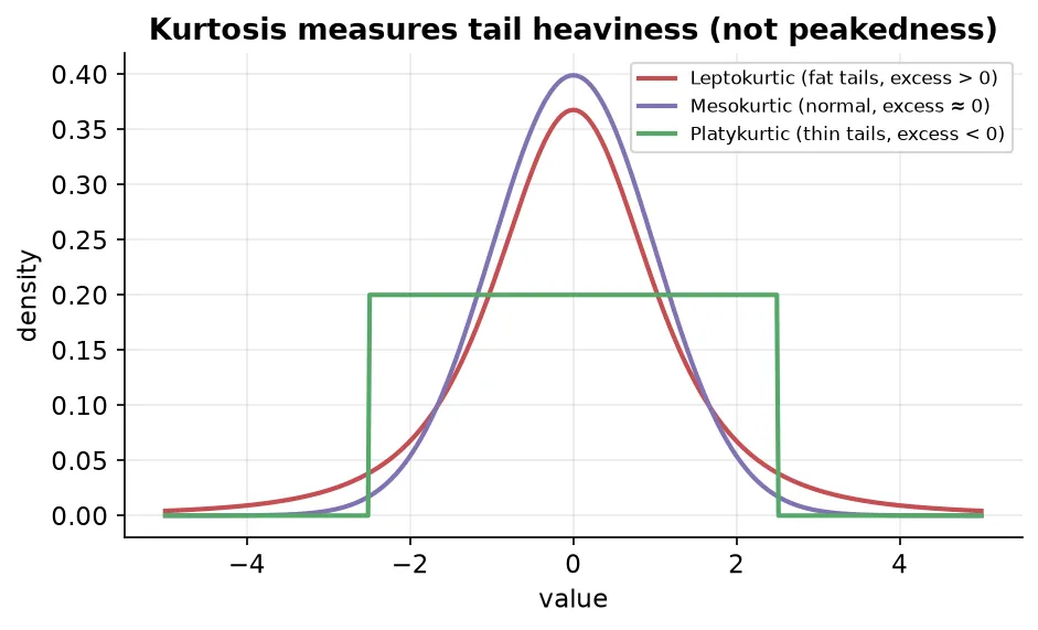
Distributions in these families can share the same mean, standard deviation, and skewness; the only difference is tail fatness.

Where kurtosis is used: finance

In finance there is a term “kurtosis risk”, the risk of extreme outcomes (fat tails) in the returns of an asset or portfolio. A highly volatile mutual fund with a leptokurtic return distribution can produce sudden large gains or losses. This is closely tied to the idea of tail events: rare events with low probability that, when they occur, hit hard and fast.

---

Checking if data is normally distributed

Before applying transformations, you need to know whether a column is already normal. Three common methods:

Method	How
Visual inspection	plot a histogram or a KDE/density plot and eyeball the shape
Skewness value	run df['col'].skew(); near 0 is symmetric, far from 0 is skewed
QQ plot	compare your data against a theoretical normal distribution graphically

The QQ plot is the most reliable and most-used of these, so it deserves its own section.

---

QQ plot (Quantile-Quantile plot)

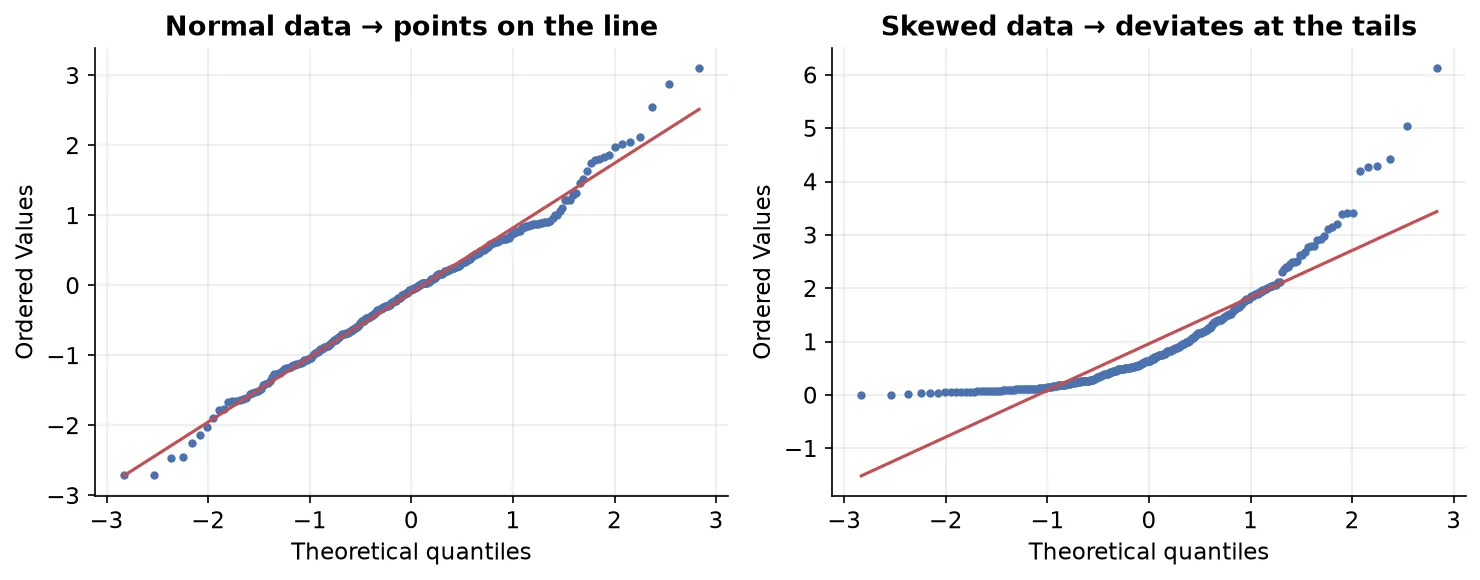
A QQ plot is a graphical tool that compares two distributions by plotting their quantiles against each other. Most often it checks whether your data follows a normal distribution.

How it is built

1. Generate a theoretical distribution (for a normal check, a standard normal with mean 0, sd 1, e.g. 1000 points).
2. Sort your actual data.
3. Compute matching percentiles/quantiles of both, and plot theoretical quantiles on the x-axis against your data’s quantiles on the y-axis.
4. Draw a reference line (usually 45°).

How to read it

• If the points lie along the straight line, the two distributions match, so your data is (approximately) normal.
• Tails are where deviations show up most. Points drifting off the line at the ends signal skew.
• Right-skewed data pulls away from the line at the top; the more it deviates, the less normal it is.

In code

statsmodels’ qqplot(data, line='45') builds it automatically: it generates the theoretical normal, does the sorting and percentile work, and fits the 45° line. Options for the reference line include 45-degree, standardized, regression, and quartile fits.

QQ plots are not just for the normal

By definition, a QQ plot compares any two distributions. Pass a theoretical uniform (or Pareto, log-normal, etc.) as the comparison distribution, and the QQ plot will tell you whether your data matches that shape. Points on the line means a match.

---

Summary

1. Skewness (3rd moment) measures asymmetry; positive skew has a long right tail (mode < median < mean), negative skew a long left tail. |value| < 0.5 is roughly symmetric, > 1 is highly skewed.
2. Kurtosis (4th moment) measures tail heaviness, not peakedness; excess kurtosis compares against the normal (leptokurtic > 0, mesokurtic ≈ 0, platykurtic < 0).
3. Check normality via visual inspection, the skewness value, and most reliably the QQ plot.
4. A QQ plot plots theoretical vs sample quantiles; points on the 45° line mean a match, and it works against any reference distribution, not just the normal.

---

Continues to

When data isn’t normal, we either model it with another distribution or reshape it. That’s the subject of non-Gaussian distributions and transformations.