P-values and T-tests

Where this fits

Continues from Hypothesis Testing. That note used the rejection-region approach, which only gives a yes/no answer. Here we learn the p-value approach, which also measures the strength of the evidence, and then apply it through the three main t-tests.

---

What is a p-value?

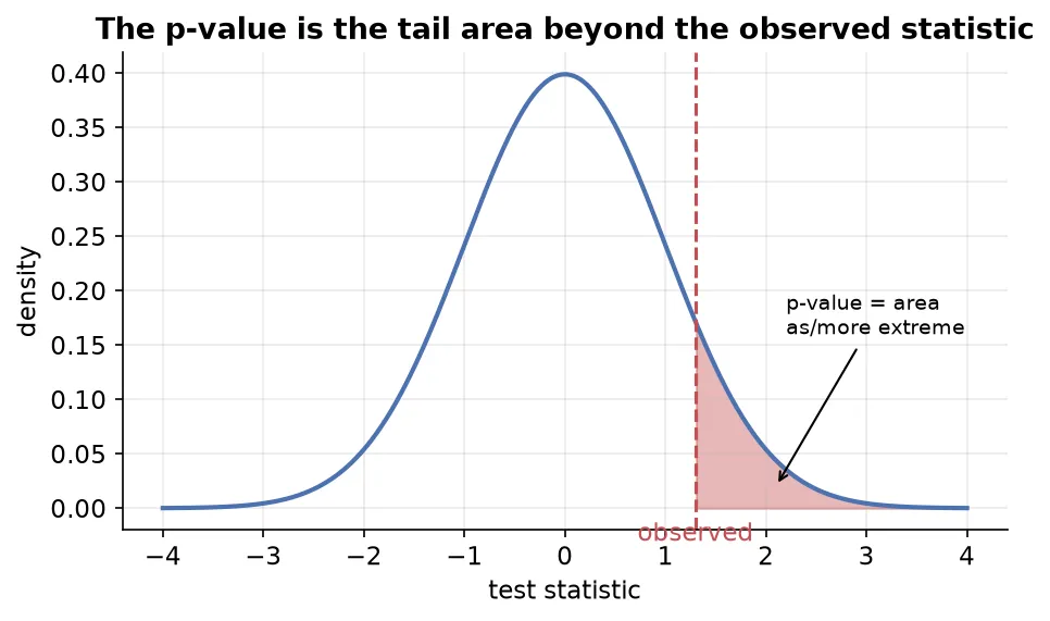
Definition

The p-value is the probability of getting a sample as or more extreme than our own sample, given that the null hypothesis is true.

“More extreme” means “providing more evidence against $H_0$”.

Building intuition with a coin

Is a coin fair?

Toss a coin 100 times and count heads. This follows a binomial distribution, and its PMF is roughly bell-shaped, peaking at 50 heads.

• $H_0$: the coin is fair, $P(\text{head}) = P(\text{tail})$.
• $H_1$: the coin is rigged, $P(\text{head}) > P(\text{tail})$.

You run the experiment and get 53 heads. The p-value is the probability of getting 53 or more heads, which is the area to the right of 53. That area ≈ 0.30.

Result	p-value (area to the right)	Meaning
53 heads	≈ 0.30	weak evidence; happens often for a fair coin
60 heads	≈ 0.02	stronger evidence
80 heads	≈ 0	extremely unlikely for a fair coin

So the p-value tells you how likely your (or a more extreme) result is assuming the null is true. A tiny p-value means your result would be very surprising under $H_0$, which is strong evidence against it.

Decision rule

Rule of thumb

If p-value $\le \alpha$ (usually 0.05), reject $H_0$. Otherwise, fail to reject $H_0$.

When you don’t have a fixed $\alpha$, a rough guide:

p-value	Evidence against $H_0$
$\le 0.01$	strong → reject
between 0.01 and 0.05	moderate → reject
between 0.05 and 0.10	weak → investigate more
$> 0.10$	insufficient → fail to reject

Why p-value beats the rejection-region approach

The rejection-region approach only says “reject or not”. The p-value also encodes how strong the evidence is: a p-value of 0.001 is far stronger evidence against $H_0$ than 0.049, even though both lead to rejection. That extra information is why the p-value approach is preferred.

---

P-value with a Z-test

Same setup as the Z-test in Hypothesis Testing, but now we read off a p-value instead of comparing to a critical value.

Training program (one-tailed)

$H_0: \mu = 50$, $H_1: \mu > 50$, $\bar{x} = 53$, $\sigma = 5$, $n = 30$. $Z = \frac{53 - 50}{5/\sqrt{30}} \approx 4.10$ The p-value is the area to the right of 4.10 (because $H_1$ is $>$). Using a Z-table (or 1 - norm.cdf(4.10)), this area ≈ 0.00004. Since $0.00004 \le 0.05$, reject $H_0$.

Lays packet (two-tailed)

$H_0: \mu = 50$, $H_1: \mu \ne 50$. Compute $Z \approx -1.26$. For a two-tailed test, take the area to the left of $-1.26$ and double it: $2 \times 0.103 = 0.206$. Since $0.206 > 0.05$, fail to reject $H_0$.

One-tailed vs two-tailed p-values

For a two-tailed test, double the one-sided tail area. For a one-tailed test, use the single tail area directly.

---

The t-test

A t-test is very similar to a Z-test, with one key difference.

	Z-test	T-test
Population $\sigma$	known	unknown (use sample $s$)
Distribution used	normal	Student’s t-distribution
Good for	large samples	works well for small samples too

Because we substitute the sample standard deviation $s$ for the unknown $\sigma$, we use the t-distribution (see Confidence Intervals for its properties: fatter tails, parameter = degrees of freedom).

There are three t-tests, each for a different situation.

---

1. One-sample t-test

Checks whether a single sample’s mean differs from a known population mean.

Assumptions: normality (of the population/sample), independent observations, random sampling, and $\sigma$ unknown.

Chocolate bar weight

Population claim $\mu = 50$ g. Sample of $n = 25$ bars: $\bar{x} = 49.7$, $s = 1.2$. Is the mean different from 50? ($\alpha = 0.05$.)

• $H_0: \mu = 50$, $H_1: \mu \ne 50$.
• Check normality first with a Shapiro-Wilk test on the 25 values (if its p-value > 0.05, the data is approximately normal).
• Compute $t = \dfrac{49.7 - 50}{1.2/\sqrt{25}} = -1.25$, degrees of freedom $= 24$.
• Get the two-tailed p-value from the t-distribution. It’s > 0.05, so fail to reject $H_0$.

Shapiro-Wilk test

A separate hypothesis test whose $H_0$ is “the data is normally distributed”. If its p-value > 0.05, treat the data as normal. Useful for checking the normality assumption before a t-test.

Titanic age

Claim: mean age of all 1309 passengers is < 35. Draw a sample of 25 ages, check normality (Shapiro-Wilk), run a one-tailed one-sample t-test with scipy.stats.ttest_1samp(sample, popmean=35), halve the p-value (one-tailed), and compare to $\alpha$.

---

2. Independent two-sample t-test

Compares the means of two independent groups.

Assumptions: independence of observations, normality within each group, and equal variances across the two groups.

Levene’s test

A separate test whose $H_0$ is “the two groups have equal variances”. Run it (or an F-test) to check the equal-variance assumption. If variances are unequal, use Welch’s t-test instead.

Desktop vs mobile dwell time

A site owner claims average time on desktop and mobile is the same. Collect 30 desktop users ($\bar{x} = 18.5$, $s = 3.5$) and 30 mobile users ($\bar{x} = 14.3$, $s = 2.7$). ($\alpha = 0.05$.)

• $H_0: \mu_{\text{desktop}} - \mu_{\text{mobile}} = 0$, $H_1: \ne 0$.
• Check normality of each group (Shapiro-Wilk) and equal variance (Levene).
• Use scipy.stats.ttest_ind(group1, group2). The p-value comes out ≈ 0, so reject $H_0$: the two means differ.

Degrees of freedom

For the independent two-sample t-test, degrees of freedom $= n_1 + n_2 - 2$.

Titanic (age vs gender)

Claim: average age of males differs from females. Draw 25 male ages and 25 female ages, then run ttest_ind. A large p-value means we can’t conclude a difference; if so, drawing bigger samples helps because the true population means (≈ 30.6 vs 28.7) are actually close.

---

3. Paired two-sample t-test

Compares two related / dependent measurements, typically before vs after on the same subjects.

Assumptions: paired observations, independence between pairs, and normality of the differences.

Weight-loss program

Measure 15 people’s weight before and after a program.

• $H_0: \mu_{\text{before}} = \mu_{\text{after}}$, $H_1: \mu_{\text{before}} > \mu_{\text{after}}$ (weight should drop).
• Compute the difference for each person, then check that the differences are normal (Shapiro-Wilk).
• Run scipy.stats.ttest_rel(before, after) and interpret the p-value.
• The test works on the differences: $t = \dfrac{\bar{d} - 0}{s_d/\sqrt{n}}$.

Other paired scenarios

Matched or correlated groups (siblings, paired individuals) also use the paired t-test.

---

Choosing the right t-test

                Are the two sets of measurements related?
                     /                        \
                   No                          Yes
                   │                            │
        Independent two-sample          Paired two-sample
             t-test                          t-test

    Only one sample vs a known population mean?  →  One-sample t-test

---

Summary

1. The p-value is the probability of a result as or more extreme than observed, assuming $H_0$ is true; small p-values are strong evidence against $H_0$.
2. Decision rule: p-value $\le \alpha$ → reject $H_0$.
3. The p-value approach beats the rejection-region approach because it also captures the strength of evidence.
4. For a two-tailed test, double the one-sided tail area; for one-tailed, use it directly.
5. A t-test replaces the unknown $\sigma$ with the sample $s$ and uses the t-distribution.
6. One-sample t-test: sample mean vs a known population mean.
7. Independent two-sample t-test: two separate groups (check equal variance with Levene, else use Welch).
8. Paired t-test: before/after on the same subjects (test the differences).
9. Use Shapiro-Wilk to check normality assumptions before running a t-test.