Bernoulli and Binomial Distributions

Where this fits

These notes continue from the distributions arc that ended with Non-Gaussian Distributions and Transformations. Those notes covered continuous distributions (normal, uniform, log-normal, Pareto). Here we cover two closely related discrete distributions that show up constantly in machine learning classification problems, and that also become the building blocks for the Central Limit Theorem.

---

Bernoulli distribution

A Bernoulli distribution models a single random experiment with exactly two possible outcomes, usually called success (1) and failure (0).

Note

Named after the Swiss mathematician Jacob Bernoulli, who introduced it in the late 1600s. It only applies to binary outcomes.

Any single trial with a yes/no result is a Bernoulli experiment.

Experiment	Success (1)	Failure (0)
Coin toss	head	tail
Email spam classifier	spam	not spam
Rolling a die and “getting a 5”	a 5 appears (prob 1/6)	anything else (prob 5/6)

Tip

“Success” does not mean a good outcome. It is just the event you chose to label as 1. When hunting spam, spam is the “success”.

PMF of the Bernoulli distribution

The single parameter is p, the probability of success. The probability of failure is automatically $1 - p$.

$$P(X = x) = p^{x}\,(1-p)^{1-x}, \qquad x \in \{0, 1\}$$

Fair coin

Let head = success with $p = 1/2$.

• $P(X=1) = (1/2)^1 (1/2)^0 = 1/2$
• $P(X=0) = (1/2)^0 (1/2)^1 = 1/2$

The graph

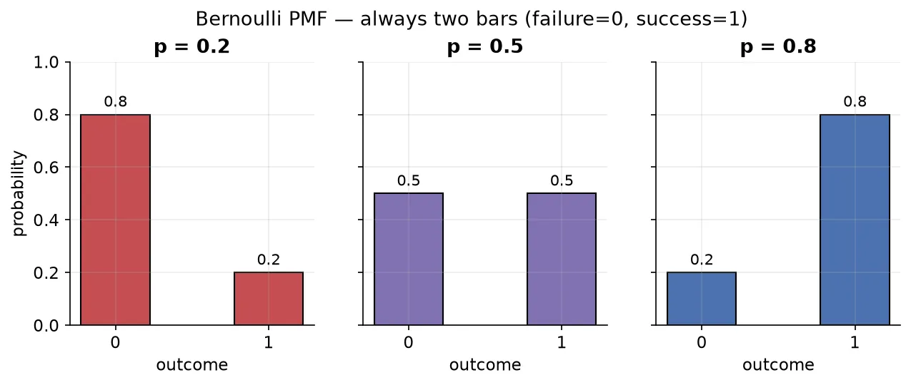
The PMF graph is always just two bars, one at 0 and one at 1. Their heights are $1-p$ and $p$.

Why it matters in ML

The Bernoulli distribution appears everywhere in classification. Any time the target/output is a class (yes/no, 1/0, spam/not-spam), the outcome can be treated as Bernoulli. Algorithms such as logistic regression, SVM, decision trees, and especially Naive Bayes lean on this assumption internally.

On its own it is simple; its real power is as the seed for the binomial distribution.

---

Binomial distribution

A binomial distribution describes the number of successes in a fixed number of independent Bernoulli trials, where the probability of success is constant on every trial.

Simply put: run a Bernoulli trial n times and count how many successes you get.

Important

If $n = 1$ (a single trial), the binomial distribution becomes the Bernoulli distribution.

Two parameters

Parameter	Meaning
$n$	number of trials
$p$	probability of success on each trial

Trials must be independent

The trials cannot influence each other. If you survey 10 students about a course and one student’s opinion sways another’s, the trials are no longer independent, and the binomial model breaks.

Building intuition: sample space first

Suppose 3 people watch a video and each likes it with probability $p = 1/2$. What is the probability that nobody likes it?

List the sample space (Yes/No for each of 3 people): there are $2^3 = 8$ equally likely cases.

# successes	Cases	Count	Probability
0 likes	NNN	1	1/8
1 like	YNN, NYN, NNY	3	3/8
2 likes	YYN, YNY, NYY	3	3/8
3 likes	YYY	1	1/8

As the number of trials grows, listing the sample space becomes impossible. That is where the formula helps.

PMF of the binomial distribution

$$P(X = x) = \binom{n}{x}\, p^{x}\,(1-p)^{\,n-x}$$

• $x$ = the desired number of successes.
• $\binom{n}{x} = \dfrac{n!}{x!\,(n-x)!}$ counts how many ways those successes can be arranged.
• The $p^{x}(1-p)^{n-x}$ part is exactly the Bernoulli PMF repeated; the $\binom{n}{x}$ factor accounts for the different arrangements.

2 out of 3 likes

$P(X=2) = \binom{3}{2}\left(\tfrac12\right)^2\left(\tfrac12\right)^1 = 3 \cdot \tfrac18 = \tfrac{3}{8}$ This matches the sample-space count above.

The graph and the role of p

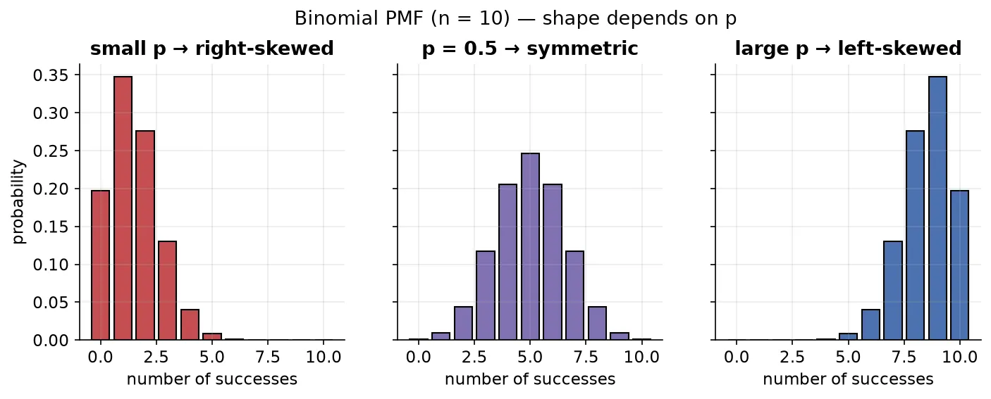
The shape of the binomial PMF depends on p:

Probability of success	Shape
$p$ high (close to 1)	left-skewed (graph shifts right)
$p \approx 0.5$	symmetric, looks like a normal distribution
$p$ low (close to 0)	right-skewed (graph shifts left)

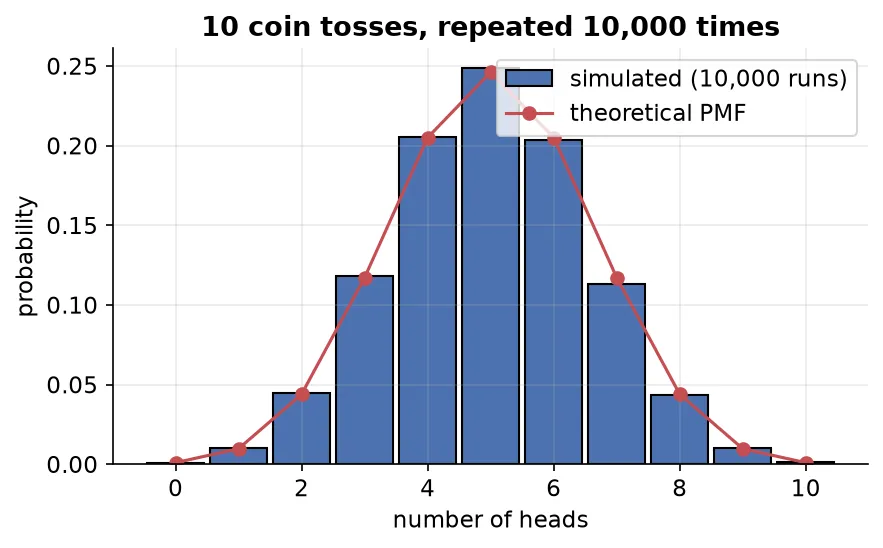
Simulating in code

import numpy as np
# 10 coin tosses, p = 0.5, repeated 1000 times
data = np.random.binomial(n=10, p=0.5, size=1000)

Each number is “how many heads in 10 tosses”. A histogram clusters around 5 (because $p = 0.5$) and looks bell-shaped. Raise p toward 1 and the whole graph shifts right; lower it toward 0 and it shifts left.

Criteria for a binomial distribution

An experiment is binomial only if all of these hold:

1. A fixed number of trials, $n$.
2. Each trial has a binary outcome (success/failure).
3. Trials are independent.
4. The probability of success $p$ is constant across trials.

Where it matters in ML

The binomial distribution appears in logistic regression and other models that reason about counts of binary events. In short: repeat a Bernoulli experiment $n$ times and its behavior follows the binomial distribution.

---

Summary

1. Bernoulli models a single binary trial with parameter $p$; its PMF is $p^x(1-p)^{1-x}$, and its graph is two bars.
2. It is the natural model for a single classification outcome (yes/no).
3. Binomial counts successes over $n$ independent Bernoulli trials with parameters $n$ and $p$; its PMF is $\binom{n}{x}p^x(1-p)^{n-x}$.
4. With $n = 1$, binomial reduces to Bernoulli.
5. The binomial shape is right-skewed for small $p$, symmetric near $p = 0.5$, and left-skewed for large $p$.
6. A valid binomial needs fixed trials, binary outcomes, independence, and constant $p$.