Hypothesis Testing

Where this fits

Continues from Confidence Intervals. Hypothesis testing is one of the most important topics in inferential statistics and a favorite in data-science and data-analyst interviews. This note covers the why, the core vocabulary, and the rejection-region approach. The follow-up, P-values and T-tests, covers the more refined p-value approach and specific tests.

---

Why hypothesis testing exists

We often have an idea (a hypothesis) and want to check whether the data supports it.

YouTube video style (hypothetical)

Average view duration is 6 minutes. You think a new shooting style (standing in front of the screen) will increase it. You shoot one video and it runs 13 minutes. Can you conclude the new style works? No. A single result could be luck (a trending topic that day, etc.). You need many samples and a formal test.

Lays packet weight

A packet claims 50 g. A consumer watchdog suspects it is not exactly 50 g. They weigh a random sample of packets and test the claim.

Hypothesis testing lets us make probabilistic statements about population parameters from sample data. It is used to compare treatments, compare group means/proportions, analyze relationships, check goodness of fit, and run A/B tests.

---

The two hypotheses

Every test starts with two competing statements.

Hypothesis	Symbol	What it says
Null hypothesis	$H_0$	Nothing new is happening; the status quo holds. Usually contains an equality.
Alternate hypothesis	$H_1$ or $H_A$	The opposite of the null; the effect the researcher wants to demonstrate.

They are mutually exclusive: exactly one will be supported at the end.

Rule of thumb for choosing the null

$H_0$ always says “nothing changed”. You changed the video style but the average duration is still 6 minutes. You opened the chips packet but the weight is still exactly 50 g.

Writing them formally

YouTube: $H_0: \mu = 6$ min, $H_1: \mu > 6$ min. Lays: $H_0: \mu = 50$ g, $H_1: \mu \ne 50$ g.

What the whole test does

We collect evidence against the null hypothesis in the hope of rejecting it.

Failing to reject ≠ proving true

Not being able to reject $H_0$ does not prove $H_0$ is true. It only means we lacked enough evidence to reject it.

Courtroom analogy

• $H_0$: the accused is innocent (“no crime”).
• $H_1$: the accused is guilty.
• The lawyer (like the researcher) presents evidence to convince the judge of guilt.
• If the lawyer fails to bring enough evidence, it does not prove the accused is innocent, it just means guilt wasn’t established.

---

Significance level ($\alpha$)

The significance level $\alpha$ is a threshold, chosen before testing. Common values are 0.05 (5%) and 0.01 (1%).

It is the probability of rejecting $H_0$ when $H_0$ is actually true (this is a Type I error, covered below). If $\alpha = 0.05$, then in the long run about 5 out of 100 true nulls would be wrongly rejected.

Note

$\alpha$ must be fixed in advance, otherwise you have no threshold against which to decide whether to reject the null.

---

The rejection-region approach (step by step)

This is the first, most basic technique. The general flow:

1. Formulate $H_0$ and $H_1$.
2. Choose the significance level $\alpha$ (e.g. 0.05).
3. Check assumptions about the data (e.g. normality, known $\sigma$) to pick the right test.
4. Decide the test (Z-test if $\sigma$ known and data normal; t-test if $\sigma$ unknown; chi-square for categorical, etc.).
5. Select the test statistic and compute it.
6. Conduct the test: compare the statistic against the critical value(s) to see if it lands in the rejection region.
7. Conclusion: reject $H_0$, or fail to reject it.

---

Worked example: one-sample Z-test (rejection region)

Training program

A car factory produces on average $\mu = 50$ cars/day with $\sigma = 5$. After a training program, a sample of $n = 30$ employees shows a sample mean of $\bar{x} = 53$. Did productivity increase? Use $\alpha = 0.05$.

Step 1. $H_0: \mu = 50$, $H_1: \mu > 50$.

Step 2. $\alpha = 0.05$.

Step 3. $n = 30 \ge 30$ (CLT → normality holds), and $\sigma$ is known → use a Z-test.

Step 5–6. Compute the Z statistic: $Z = \frac{\bar{x} - \mu}{\sigma/\sqrt{n}} = \frac{53 - 50}{5/\sqrt{30}} \approx 3.28$

Because $H_1$ is $\mu > 50$, this is a one-tailed (right-tailed) test. Put all of $\alpha = 0.05$ in the right tail. The critical value is $z = 1.645$.

Step 7. $3.28 > 1.645$, so the statistic lands in the rejection region. We reject $H_0$: the training program significantly increased productivity.

            |          rejection region (α = 0.05)
            |                 ┌───────
   ─────────┴─────────────────┤
            0               1.645   3.28 ✗ (falls here → reject H0)

---

One-tailed vs two-tailed tests

The alternate hypothesis decides which one you use.

$H_1$ contains	Test type	Rejection region
$>$ or $<$ (a direction)	one-tailed (one-sided)	all $\alpha$ in one tail
$\ne$ (just “different”)	two-tailed (two-sided)	$\alpha/2$ in each tail

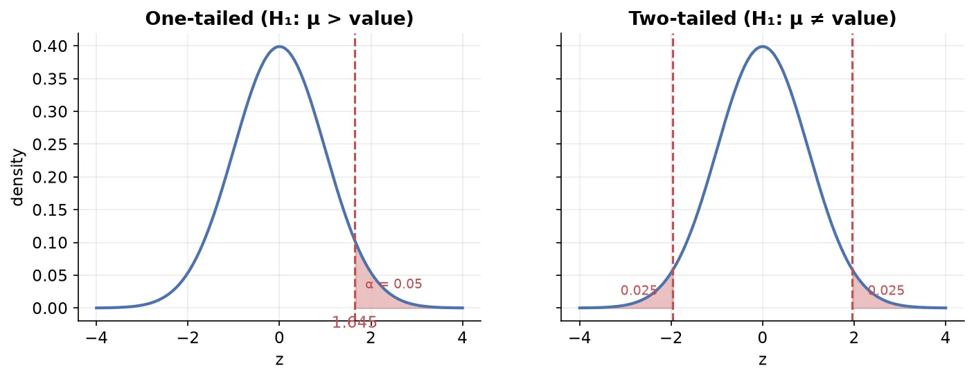
Lays packet (two-tailed)

$H_0: \mu = 50$, $H_1: \mu \ne 50$. With $\alpha = 0.05$, put 0.025 in each tail, giving critical values $\pm 1.96$. Compute $Z = \dfrac{49 - 50}{4/\sqrt{40}} \approx -1.58$. Since $-1.58$ lies between $-1.96$ and $1.96$ (the no-rejection region), we fail to reject $H_0$. There isn’t enough evidence that the weight differs from 50 g.

---

Type I and Type II errors

Because we decide from a sample, we can be wrong in two ways.

	$H_0$ is true	$H_0$ is false
Reject $H_0$	Type I error (false positive), prob $\alpha$	correct
Fail to reject $H_0$	correct	Type II error (false negative), prob $\beta$

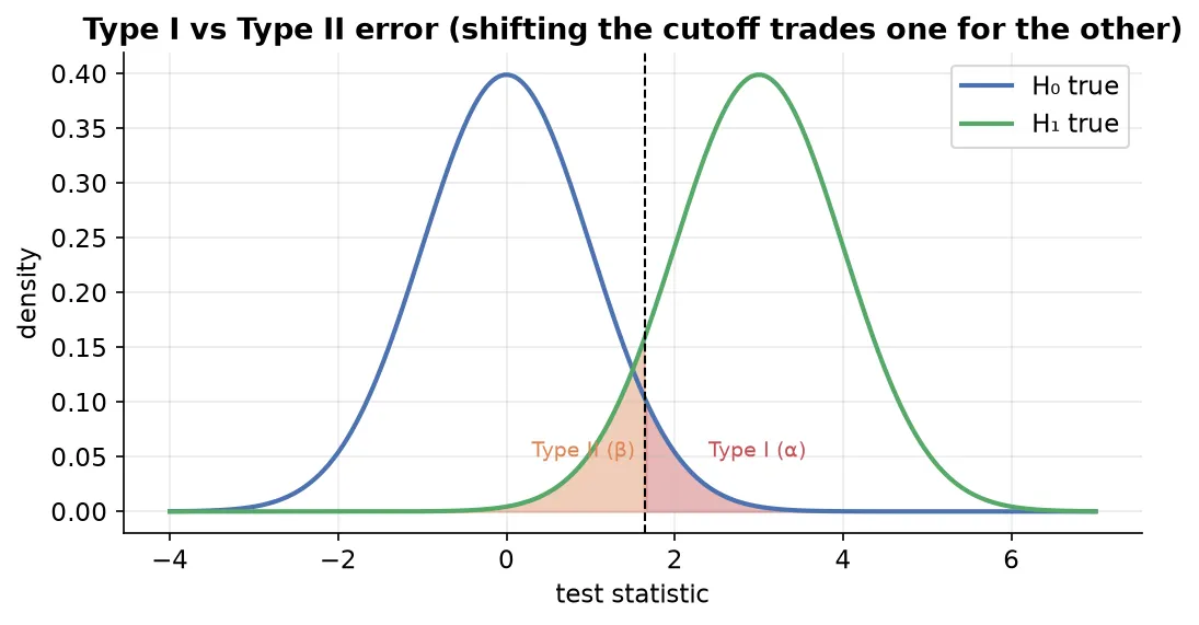
• Type I error (false positive): rejecting a true null. Example: the innocent person gets convicted. Its probability is $\alpha$.
• Type II error (false negative): failing to reject a false null. Example: the guilty person walks free. Its probability is $\beta$.
• Power of the test $= 1 - \beta$.

The trade-off

Lowering $\alpha$ shrinks the rejection region and grows the “fail to reject” region. That reduces Type I errors but increases Type II errors, and vice versa. You cannot minimize both at once; you strike a balance (which is why 0.05 is a common default).

---

How $\alpha$ shapes the regions (intuition)

Picture a two-tailed test. The white middle region is “fail to reject”; the shaded tails are “reject”.

• Decrease $\alpha$ (e.g. 0.05 → 0.01): the white region grows, so it’s harder to reject $H_0$ (fewer Type I errors).
• Increase $\alpha$: the white region shrinks, so even a true $H_0$ is more likely to be (wrongly) rejected.

The value from the Z/t table that separates the regions is the critical value; the shaded area is the rejection region.

---

The weakness of the rejection-region approach

This approach gives a binary answer (reject or not) but ignores how strong the evidence is.

Example

If the critical value is 1.96 and your statistic is 1.97, you reject; if it’s 1.95, you don’t, even though the two are almost identical. And a statistic of 15 (very strong evidence) is treated the same as one of 2 (borderline). The rejection-region approach can’t express this difference in strength.

The fix is the p-value approach, covered in P-values and T-tests.

---

Where hypothesis testing is used in ML

Use case	How
Model comparison	test whether one model’s accuracy is significantly better across CV folds (paired t-test)
Feature selection	test whether a feature is significantly related to the target (t-test, chi-square, ANOVA)
Hyperparameter tuning	compare performance across parameter settings
Checking model assumptions	test linearity/normality of residuals (e.g. for linear regression)

Libraries like scikit-learn use these tests internally; understanding them helps you use those tools wisely.

---

Summary

1. Hypothesis testing checks whether data supports an idea about a population parameter.
2. $H_0$ (null) says “nothing new”; $H_1$ (alternate) is the effect we want to show; the goal is to gather evidence against $H_0$.
3. Failing to reject $H_0$ does not prove it true.
4. $\alpha$ (significance level, often 0.05) is the pre-chosen probability of a Type I error.
5. The rejection-region approach: compute a test statistic and check if it falls beyond the critical value.
6. One-tailed tests (direction in $H_1$) put $\alpha$ in one tail; two-tailed tests ($\ne$) split it into both tails.
7. Type I = false positive (prob $\alpha$); Type II = false negative (prob $\beta$); they trade off; power $= 1 - \beta$.
8. The rejection-region approach ignores the strength of evidence, which the p-value approach fixes.