Confidence Intervals

Where this fits

Continues from Central Limit Theorem. The CLT told us the sampling distribution of the mean is normal. Here we use that fact to put a range around a population parameter, instead of guessing a single number. This is a core inferential-statistics tool and a common interview topic.

---

Revision: the vocabulary we need

Term	Meaning	Symbol
Population	the entire group of interest	—
Sample	a random, representative subset we actually measure	—
Parameter	a numeric summary of the population (unknown)	$\mu$, $\sigma$
Statistic	a numeric summary of the sample (known)	$\bar{x}$, $s$

We use a statistic (from the sample) to estimate a parameter (of the population). Parameters are usually unknown, which is the whole reason inferential statistics exists.

---

Point estimate

A point estimate is a single value, calculated from a sample, used as the best guess for an unknown population parameter.

Example

To estimate the average age of a YouTube channel’s subscribers, hold a live class, ask 100 attendees their age, and compute the sample mean (say 28). That 28 is the point estimate for the whole subscriber base.

You can make a point estimate stronger by taking many samples and averaging their means (an application of the Central Limit Theorem), but it is still a single number.

The problem with point estimates

A single number is not reliable. How can the average of 100 people exactly equal the average of 77,000?

The betting intuition

Predict Dhoni’s score today. Guess the exact run and win big, but you’ll almost never be right. Guess a range (±10 or ±20) and you’re far more likely to be correct. A range is more useful than a point.

So statisticians report a range, called a confidence interval.

---

Confidence interval and confidence level

• Confidence interval (CI): a range of values within which we expect a population parameter to lie.
• Confidence level: how sure we are that the true value lies in that interval, expressed as a percentage (commonly 95%).

Example

“The subscribers’ average age is between 25 and 32, and I am 95% confident.” Here 25–32 is the confidence interval and 95% is the confidence level.

The master formula

$$\text{CI} = \text{point estimate} \pm \text{margin of error}$$

If the point estimate is 25 and the margin of error is 4, the CI is $25 \pm 4 = [21, 29]$.

Confidence intervals are for

parameters, not statistics We always build the interval around a population quantity (like $\mu$), using sample information.

---

Interpreting the confidence level (very important)

A 95% confidence level does not mean “there is a 95% probability the mean is in this range”. The population mean is a fixed number, it does not have a probability.

Correct interpretation

If you repeat the whole experiment many times, each time drawing a fresh sample and building a fresh 95% confidence interval, then about 95% of those intervals will contain the true population parameter. Roughly 5% will miss it.

Width vs confidence trade-off

The higher the confidence level, the wider the interval.

Example

“Dhoni scores between 0 and 200, I’m 100% confident” is useless because the range is too wide. “Between 25 and 35, I’m 95% confident” is informative. A 100% confidence interval stretches from $-\infty$ to $+\infty$.

---

Procedure 1: Z-procedure (population $\sigma$ known)

Use the Z-procedure when the population standard deviation $\sigma$ is known.

Assumptions

1. The sample was drawn randomly.
2. The population standard deviation $\sigma$ is known.
3. The population is normally distributed (or the sample size is $\ge 30$, so the CLT provides normality).

The formula

$$\text{CI} = \bar{x} \pm z_{\alpha/2}\cdot\frac{\sigma}{\sqrt{n}}$$

Symbol	Meaning
$\bar{x}$	sample mean (the point estimate)
$\sigma$	population standard deviation
$n$	sample size
$z_{\alpha/2}$	the critical value from the Z-table

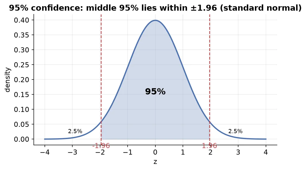
Here $\alpha$ is $1 - \text{confidence level}$. For a 95% interval, $\alpha = 0.05$, and $z_{\alpha/2} = 1.96$ (the z-value leaving 2.5% in each tail).

Where the formula comes from (intuition)

1. By the CLT, the sampling distribution of $\bar{x}$ is normal.
2. Standardize it into the standard normal variate $Z = \frac{\bar{x} - \mu}{\sigma/\sqrt{n}}$.
3. We want a range of $z$ values that captures 95% of the area, which is $[-1.96, 1.96]$.
4. Rearranging that inequality to solve for $\mu$ gives the formula above.

Common critical values

Confidence level	$z_{\alpha/2}$
90%	1.645
95%	1.96
99%	2.576

---

Procedure 2: T-procedure (population $\sigma$ unknown)

In real life you almost never know the population standard deviation. When $\sigma$ is unknown, replace it with the sample standard deviation $s$, and use the t-distribution instead of the normal.

Why not just use the normal?

Replacing $\sigma$ with $s$ adds extra uncertainty, because $s$ itself varies from sample to sample. That extra uncertainty means the standardized quantity no longer follows the normal distribution; it follows the Student’s t-distribution.

The t-distribution

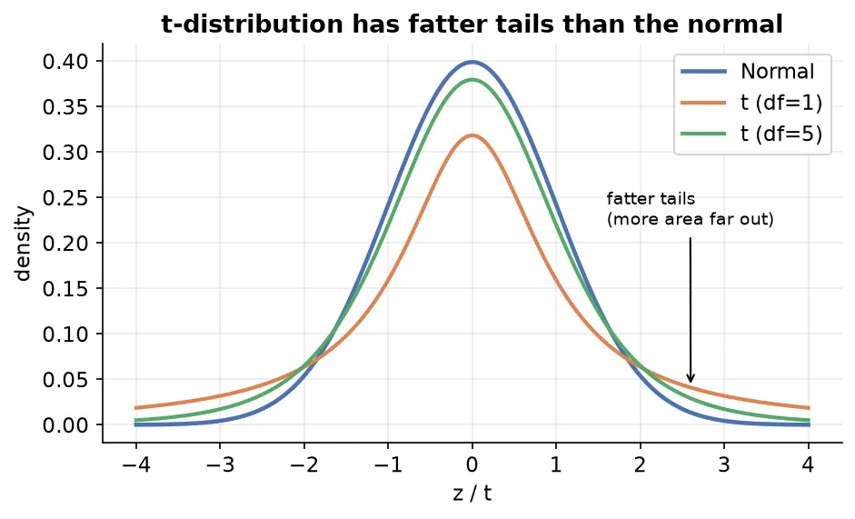
• A theoretical distribution (it does not occur in nature; it was designed to handle this uncertainty). It was published under the pen name “Student”.
• Looks like the normal distribution but with fatter tails (more area far from the center).
• Has a single parameter: degrees of freedom $= n - 1$.
• As the sample size grows, the t-distribution converges to the normal distribution.

The formula

$$\text{CI} = \bar{x} \pm t_{\alpha/2}\cdot\frac{s}{\sqrt{n}}$$

The critical value $t_{\alpha/2}$ comes from a t-table using the degrees of freedom $n-1$.

Note

For the same confidence level and small sample, $t_{\alpha/2} > z_{\alpha/2}$ (e.g. ~2.04 vs 1.96), so the t-interval is a bit wider, correctly reflecting the extra uncertainty. As $n$ grows, $t_{\alpha/2} \to z_{\alpha/2}$.

Using the wrong procedure

If you mistakenly use the Z-procedure with the sample $s$, simulations show your intervals capture the true mean only ~92% of the time even though you claimed 95%. Switching to the T-procedure restores the correct ~95% coverage.

---

Factors that affect the interval width

$$\text{CI} = \underbrace{\bar{x}}_{\text{sample mean}} \pm \underbrace{z_{\alpha/2}}_{\text{critical value}}\cdot\frac{\sigma}{\sqrt{n}}$$

Factor	Effect on width
Higher confidence level	wider interval (bigger critical value)
Larger population standard deviation	wider interval
Larger sample size $n$	narrower interval

Note

Increasing sample size helps a lot at first (going from 0 to ~30), but the benefit shrinks as $n$ grows further, because the width falls with $\sqrt{n}$, not $n$.

---

Worked example (Titanic age, T-procedure)

We want the population mean age, but we only “have” a sample.

1. Draw a random sample of 25 ages → compute sample mean $\bar{x}$ and sample std $s$.
2. $\sigma$ is unknown → use the T-procedure.
3. Degrees of freedom $= 25 - 1 = 24$; look up $t_{\alpha/2}$ for 95% ≈ 2.06.
4. Compute $\bar{x} \pm 2.06 \cdot \dfrac{s}{\sqrt{25}}$ to get the interval.
5. The true population mean age (≈ 29.7) falls inside the reported interval.

Lower the confidence level and the interval narrows but you become less sure; raise it and the interval widens.

---

Summary

1. A point estimate is a single-value guess for a population parameter; it is not reliable on its own.
2. A confidence interval gives a range, and the confidence level (e.g. 95%) states how often such intervals capture the true parameter over many repetitions.
3. $\text{CI} = \text{point estimate} \pm \text{margin of error}$.
4. Z-procedure applies when $\sigma$ is known; $\text{CI} = \bar{x} \pm z_{\alpha/2}\,\sigma/\sqrt{n}$ (95% → $z = 1.96$).
5. T-procedure applies when $\sigma$ is unknown; it uses the sample $s$ and the t-distribution (fatter tails, parameter = degrees of freedom $n-1$).
6. Interval width grows with confidence level and population spread, and shrinks with sample size.