Non-Gaussian Distributions and Transformations

Where this fits

Continues from Skewness, Kurtosis and Normality Checks. Once you know a column isn’t normal, you have two options: model it with a different distribution, or reshape it toward normal. This note covers the common non-Gaussian continuous distributions (uniform, log-normal, Pareto) and the mathematical transformations used to normalize data for distribution-sensitive algorithms.

Non-Gaussian continuous distributions

Real-world data is often not normal. Three very common non-Gaussian continuous distributions:

1. Uniform distribution

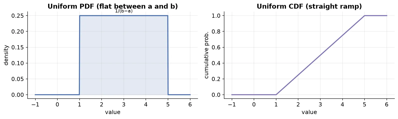
Every outcome in a range is equally likely. A fair die is the discrete version (each face has probability 1/6, so all bars are the same height).

Continuous uniform is denoted $X \sim U(a, b)$ , where a is the lower bound and b the upper bound of the range.

PDF: constant between a and b, zero elsewhere. Because the total area must be 1 and the width is $b - a$ : $f(x) = \begin{cases} \dfrac{1}{b - a} & a \le x \le b \\[6pt] 0 & \text{otherwise} \end{cases}$
CDF: 0 below a, rises steadily, and reaches 1 at b.
Skewness = 0 (it is symmetric, like the normal).

Uniform distribution PDF and CDF

Where it appears in machine learning (usually behind the scenes):

Use case	Role of uniform distribution
Random initialization	starting parameters in neural networks and k-means are drawn uniformly, so all values in a range are equally likely
Sampling	randomly selecting a representative subset (e.g. train/test split)
Random number generation	pseudo-random generators rely on it
Data augmentation	adding controlled randomness to create new data (e.g. zoomed/shifted images in CNNs)
Hyperparameter tuning	randomly searching parameter combinations

2. Log-normal distribution

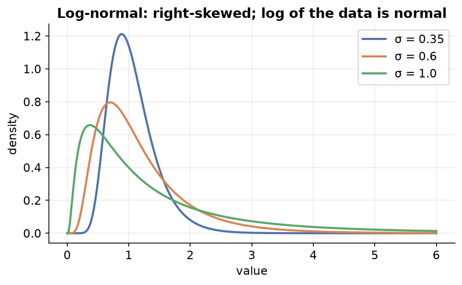
A heavy-tailed, right-skewed distribution whose logarithm is normally distributed.

Important

Not every right-skewed distribution is log-normal. Only those where taking the log of the values produces a normal distribution qualify. If X is log-normal, then ln(X) is normal.

Denoted $\text{LogNormal}(\mu, \sigma)$ , with the same two parameters as the normal (though they describe the log of the variable).
The PDF is very similar to the normal’s, essentially the normal’s cousin.

Log-normal distribution shapes

Where it appears (extremely common in internet/social applications):

Number of words in comments on YouTube, Reddit, Instagram, Facebook.
Dwell time users spend on online articles.
Length of online chess games.
Distribution of wealth/income (many people earn little, few earn a lot).

The pattern: many observations cluster at low values, and a few stretch far out to the right.

How to check for log-normal: take the log of the data, then run a QQ plot (or normality check) on the transformed values. If the transformed data is normal, the original was log-normal.

3. Pareto distribution

A special case of a power law. A power law is a functional relationship where one variable is a power of another:

y = k \, x^{-\alpha}

Its graph drops steeply then flattens into a long tail.

Pareto distribution shapes

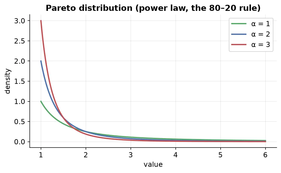
The 80–20 rule (Pareto principle): roughly 20% of causes account for 80% of effects.

Example

Wilfredo Pareto studied wealth and found that ~20% of people control ~80% of the wealth. This is the origin of the Pareto distribution.

Single parameter $\alpha$ (shape). A higher $\alpha$ gives a higher, sharper peak and thinner tail; a lower $\alpha$ gives a lower peak and fatter tail. As $\alpha \to \infty$ , the curve becomes a vertical line.
PDF: $f(x) = \dfrac{\alpha \, x_m^{\alpha}}{x^{\alpha + 1}}$ , where $x_m$ is the minimum value.
It is skewed (not symmetric).

Note

The exact 80–20 split is not universal; it depends on $\alpha$ . It is a rough guide, not a fixed law.

Where it appears: wealth/income distributions, city population vs area, file-size distribution of internet traffic (a few large files make up most of the total gigabytes).

How to detect Pareto: use a log-log plot (plot log(x) vs log(y)); a Pareto/power-law relationship shows up as a straight descending line. A QQ plot against a theoretical Pareto also works.

Mathematical transformations

Goal: convert a non-normal distribution into a (more) normal one, because several ML algorithms (linear regression, logistic regression, KNN) perform better on normally distributed data.

A transformation applies a mathematical function to a column to reshape its distribution.

Note

It is not a strict rule that normal data always helps. Whether it improves results depends on the algorithm. Tree-based models like decision trees are unaffected by the distribution; linear models are affected.

In scikit-learn, transformations live in two classes:

              scikit-learn transformers
              /            |            \
     FunctionTransformer  PowerTransformer  QuantileTransformer
       (log, reciprocal,   (Box-Cox,          (rarely used)
        square, sqrt,       Yeo-Johnson)
        custom)

FunctionTransformer transforms

Apply any function you like via FunctionTransformer(func=...).

Transform	Formula	Best for
Log	$\log(x)$	right-skewed data
Reciprocal	$1/x$	reverses order (big↔small); situational
Square	$x^2$	left-skewed data
Square root	$\sqrt{x}$	mildly right-skewed; try and check

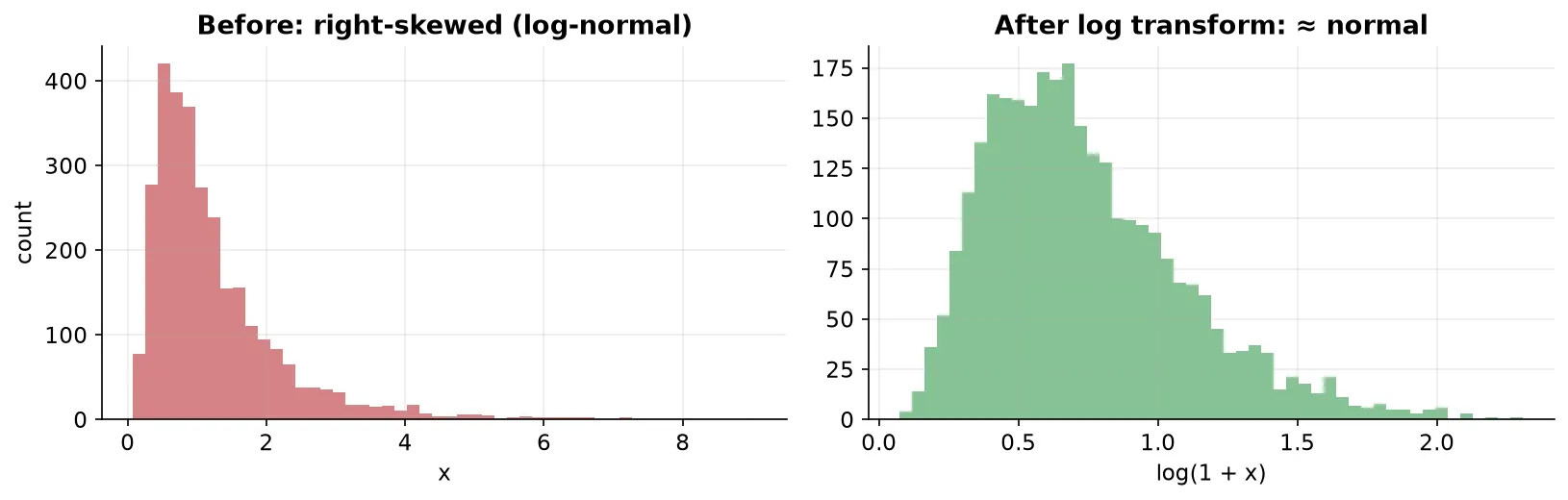
Log transform is the go-to for right-skewed data. It pulls in large values and centers the distribution. On a log scale, distant points come closer and look more linear, helping linear models.
- np.log fails on zeros/negatives. Use np.log1p, which computes $\log(1 + x)$ , so zeros are safe. If your data has no zeros, plain log is fine too.

Log transform turns right-skewed data into near-normal

There is no one-size-fits-all; try each transform and keep whichever gives the best result. You can even define a fully custom function ( $x^2 + 2x$ , a sine, etc.).

Titanic (Age + Fare → Survived)

Fare is right-skewed, Age is roughly normal. Applying a log transform to Fare and refitting logistic regression improved accuracy, while decision tree accuracy stayed the same (trees ignore distribution). Forcing a log transform on the near-normal Age actually hurt results, so a ColumnTransformer was used to transform only Fare and pass Age through unchanged. Cross-validation confirmed the improvement was real.

PowerTransformer transforms

PowerTransformer finds the best power to raise data to (via a parameter $\lambda$ , “lambda”) so the result is as normal as possible. Two methods:

Method	Data requirement	Notes
Box-Cox	strictly positive (no zero, no negative)	classic; a small constant can be added to handle zeros
Yeo-Johnson	works with positive, zero, and negative data	default in scikit-learn; often the better performer

Internally, a lambda is estimated per column (using maximum likelihood), and each value is raised to that power to transform it.
By default PowerTransformer also applies zero-mean, unit-variance standardization (standardize=True), so you usually do not need to scale separately.
Understanding what it does (map to a normal shape) is enough at this level; the deep how belongs to advanced (maximum likelihood / Bayesian) statistics.

Concrete strength dataset

A regression problem with several non-normal input columns. Baseline linear regression gave an R² (cross-validated) around 0.46. Applying Box-Cox (with a tiny constant added to zero-valued columns) raised it to about 0.66. Applying Yeo-Johnson raised it further to about 0.68. Plotting each column before vs after showed most columns becoming much closer to normal (though bimodal columns cannot be fully fixed by a single transform).

Practical workflow: check which columns are non-normal, apply PowerTransformer (try both Box-Cox and Yeo-Johnson), compare via cross-validation, and keep whatever performs best. It is essentially parameter tuning.

Summary

Common non-Gaussian distributions: uniform (equal likelihood over a range, skew 0), log-normal (right-skewed, its log is normal), and Pareto (a power law, the 80–20 rule).
Detect them by transforming and re-checking normality (log for log-normal) or with tailored plots (log-log plot / QQ plot for Pareto).
Transformations reshape non-normal data toward normal to help distribution-sensitive algorithms (linear/logistic regression, KNN); tree models are unaffected.
FunctionTransformer applies log (right-skew), square (left-skew), reciprocal, sqrt, or custom functions; log is the workhorse (use np.log1p for zeros).
PowerTransformer estimates the best power automatically: Box-Cox (positive data only) and Yeo-Johnson (handles zero/negative, the usual default).
There is no universal best transform, try several and validate with cross-validation.

Continues to

That completes the distributions arc. The story now shifts to two key discrete distributions in Bernoulli and Binomial Distributions, which open the door to inferential statistics.