Foundations and Central Tendency

What is statistics?

Statistics is the science of collecting, organizing, summarizing, and drawing conclusions from data. We use it to describe what happened in the past and to make predictions about the future.

Statistics has two main branches.

Branch	What it does	Simple idea
Descriptive	Summarizes and describes the data you already have	Studying past data
Inferential	Uses a small piece of data to make predictions about a larger group	Making predictions

• Descriptive statistics: you are given some data and you generate a description, or summary, of it. This includes mean, median, standard deviation, the five-number summary, and graphs. You only describe what is in front of you and make no predictions.
• Inferential statistics: you use the data you have to infer something about a much bigger group you cannot fully measure. This is more advanced and covers Hypothesis Testing, Confidence Intervals, ANOVA, and regression.

---

Population vs sample

This is one of the most important foundational ideas.

• Population: the entire group you care about, meaning every single individual in it.
• Sample: a subset of the population that you actually measure.

We need samples because the population is often too large to measure fully.

Example

To find the average salary in India with 140 crore people, you cannot ask every single person. Instead you pick, say, 50,000 people from different states, ages, and genders, calculate their average, and infer the population average from it.

More examples follow.

• All cricket fans form a population; the fans physically in the stadium form a sample.
• All students enrolled in a college, whether online, offline, or distance, form a population; only those physically attending lectures form a sample.

Rules for a good sample

For your inference to be trustworthy, the sample must be:

1. Large enough, because a tiny sample cannot represent a huge population well.
2. Random, with no bias, so every individual has a fair chance of being picked.
3. Representative, so every variation in the population such as state, age, and gender appears in the sample.

If the sample is built poorly, every prediction you make about the population will be wrong.

---

Types of data

Knowing the type of each column tells you which concepts and graphs you can apply.

                        DATA
                  /              \
          CATEGORICAL          NUMERICAL
          /        \            /        \
      Nominal    Ordinal   Discrete   Continuous

Categorical data

Categorical data holds categories or labels.

• Nominal: categories with no order.
  • Example: gender (Male, Female), state (Haryana, Bihar, Maharashtra).
• Ordinal: categories that have an order or ranking.
  • Example: feedback (Bad, then Average, then Good).

Numerical data

Numerical data holds numbers.

• Discrete: only whole numbers, because you count it.
  • Example: number of children, number of cars.
• Continuous: any value, including decimals, because you measure it.
  • Example: weight (35.3 kg), height (172.4 cm).

Tip

Always ask: is this column categorical or numerical? If categorical, is it nominal or ordinal? If numerical, is it discrete or continuous? This drives every analysis decision.

---

Measure of central tendency

A measure of central tendency is a single value that represents the center of a data set, meaning the typical value.

Mean (average)

Add all values and divide by how many there are.

$$3 + 4 + 1 + 2 + 5 = 15 \quad\Rightarrow\quad \frac{15}{5} = 3$$

So the mean is 3.

Population mean and sample mean use the same arithmetic but different symbols and meaning.

• Population mean: $\mu = \dfrac{\sum x_i}{N}$, where $N$ is the size of the population.
• Sample mean: $\bar{x} = \dfrac{\sum x_i}{n}$, where $n$ is the size of the sample.

Always know whether your data is a population or a sample, because the two can give different results.

The big flaw of the mean is that it is sensitive to outliers.

Example

A classroom earns around 30,000 per month. One student lands a package of lakhs. The mean salary shoots up to lakhs and no longer represents the typical student. One extreme value, called an outlier, shifts the mean badly.

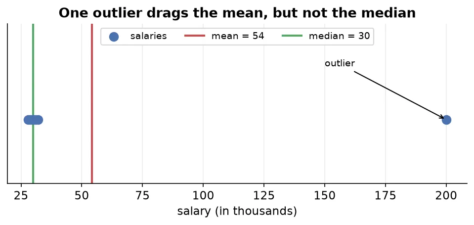
If your data has outliers, the mean is a poor measure.

Median

The median is the middle value when the data is arranged in order.

Steps:

1. Sort the data in ascending or descending order.
2. If the count is odd, the middle value is the median.
3. If the count is even, take the average of the two middle values.

The median beats the mean for outliers because, when you sort, an extreme value goes to the far end and never to the middle. So it cannot distort the median.

Example

If Bill Gates stands in a salary line, he stands at the very end. The middle person still represents the class correctly.

Use the median when outliers are present.

Mode

The mode is the most frequent value in the data set.

It is most useful for categorical data, where it shows which category appears most often, and for discrete numerical data.

Example

Ask every student which state they are from, then count each state. The state appearing most is the mode.

Weighted mean

Instead of treating all values equally, assign each one a weight, meaning an importance.

$$\text{Weighted mean} = \frac{\sum (\text{value} \times \text{weight})}{\sum \text{weights}}$$

Example

Three model predictions weighted 0.2, 0.3, and 0.5 are combined by importance.

Trimmed mean

Remove a fixed percentage of the smallest and largest values, then take the mean of the rest. This reduces the effect of outliers.

Example

With a 20 percent trimmed mean, drop the bottom 20 percent and top 20 percent of values, then average what remains. The trimming percentage is how much you cut from each end.

Quick summary

Measure	Best for	Weakness
Mean	clean numerical data	ruined by outliers
Median	data with outliers	ignores exact values
Mode	categorical or discrete data	not useful for continuous data

---

Measure of dispersion (spread)

Central tendency alone is not enough. Two different data sets can have the same mean.

Data A: -5,  0,  5     ->  mean = 0
Data B: -10, 0, 10     ->  mean = 0

Both have the same center, but B is more spread out. A measure of dispersion tells us how spread out the data is around its center.

Range

Range = Maximum value - Minimum value

The range is easy to compute, but it is heavily affected by outliers, since one extreme point inflates it. It is rarely reliable on its own.

Variance

Variance is the average of the squared differences between each point and the mean. It tells you how far values are from the mean on average.

• Sample variance: $s^2 = \dfrac{\sum (x_i - \bar{x})^2}{n - 1}$
• Population variance: $\sigma^2 = \dfrac{\sum (x_i - \mu)^2}{N}$

Worked example with data 3, 2, 1, 5, 4 and mean 3:

$$\begin{aligned} &(3-3)^2 + (2-3)^2 + (1-3)^2 + (5-3)^2 + (4-3)^2 \\ &= 0 + 1 + 4 + 4 + 1 = 10 \\ &\frac{10}{5} = 2 \end{aligned}$$

Key points about variance:

• It is proportional to the spread, so a bigger spread gives a bigger variance, but it is not the spread itself.
• It is prone to outliers, because squaring differences makes far points dominate.
• The denominator is n - 1 for samples and N for population. The reason belongs to inferential statistics.
• Its unit is squared. If data is in LPA, variance is in LPA squared, which is hard to interpret. The next measure fixes this.

Standard deviation

$$\text{Standard deviation} = \sqrt{\text{Variance}}$$

Example

If variance is 2, standard deviation is 1.41.

Standard deviation has the same unit as the original data, not squared, so it is directly interpretable. It tells you, on average, how far values lie from the mean.

Mean absolute deviation (MAD)

Instead of squaring, take the absolute distance from the mean and average it. It uses the same unit as the data. Its limitation appears in inferential statistics, because you cannot easily infer the population MAD from a sample.

Coefficient of variation (CV)

$$CV = \frac{\text{Standard deviation}}{\text{Mean}} \times 100\%$$

The coefficient of variation lets you compare the variability of two different columns.

Example

You cannot directly compare the spread of salary and experience, because they have different units and scales. CV normalizes spread relative to each column’s own mean, giving a unit-free number you can compare.

• A larger CV means the data is more spread out relative to its mean.
• A smaller CV means the data is more tightly concentrated around its mean.

---

Summary

1. Statistics describes data through descriptive methods and predicts from data through inferential methods.
2. A population is everyone; a sample is a representative subset that must be large, random, and representative.
3. Data types are categorical, meaning nominal or ordinal, and numerical, meaning discrete or continuous.
4. Central tendency uses the mean, which is sensitive to outliers, the median, which is robust, and the mode, which suits categories.
5. Dispersion uses range, variance, standard deviation, which shares the data’s unit, mean absolute deviation, and coefficient of variation, which compares across columns.

---

Continues to

Center and spread give you two numbers. To see the full shape of a column you need its quantiles, covered in Quantiles and Box Plots.